PCh7 Lec4

(3/25/20, bes)

Sec 7.3: 3D Rotation

The following expects that you have your textbook open to section 7.3 and are reading long...

Okay, just like every other quantum system that we have been working with, we must define the Hamiltonian operator (total energy operator), find an acceptable solution for the eigenfunctions, and then determine the eigenvalues (total energy). Because we are working in 3D, it is not real convenient to use x, y, and z, so like 2D rotation, we are shifting over to define the system in terms of spherical polar coordinates (spc).

At this stage of QM, sometimes introduces a new term called the Laplacian, an upside down triangle. Although your text does not do this until the hydrogen atom (Ch 9), but here is a quick glimpse:

Note that the entire 3D rotation Schrodinger Equation is shown in your text in eq. 7.17. Spend a little time comparing eq. 7.17 to the Hamiltonian equation above...note to following:

- the 1/r^2 has been factored out of the expression in eq. 7.17,

- "m" has been replaced with "μ" the reduced mass in eq. 7.17, and

- the potential energy term is zero.

Your text continues with a short discussion of how one might solve for the eigenvalues; this discussion involves the "separation of variables," which means instead of having one function Υ(θ, φ) dependent on both θ and φ, we now have a function that is a product of θ and φ, Θ(θ)*Φ(φ) (see eq. 7.20). Your text does not go into much more detail before providing you with the solution to the eigenfunction, the "spherical harmonics." Like the previous 2D rotation solution was given to you as the Hermite polynomials, hereto the solution is just stated to be the spherical harmonics.

Some important issues come out of this discussion:

1) The 3D rotation solution is kind of like the 2D + 1D. In the 2D solution, the integer m_l = 0, ±1, ±2, ±3, ..., so the 3D solution contains this integer as well as one more, l = 0, 1, 2, 3, ... This is not a whole lot different than when we discussed the 1D box --> "n", 3D box --> ""n_x, n_y, n_z," one integer for each dimension or as your text notes, one integer for each set of boundary conditions.

2) Even though there are two integers, the total energy is only dependent on one, l; 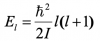, so once we take into account the relationship between the integers, ie. l = 0, 1, 2, 3, ..., but m_l = 0, thru ±l, this leads to energy levels that are degenerate. Recall, I (eye) = moment of inertia and is equal to μr², not to be confused with l (el).

l = 0 has only 1 energy level (m_l = 0)

l = 1 has only 3 energy level (m_l = -1, 0, +1)

l = 2 has only 5 energy level (m_l = -2, -1, 0, +1, +2)

l = 3 has only 7 energy level (m_l = -3, -2, -1, 0, +1, +2, +3)

Draw in your notes an energy level diagram for 3D rotation including l = 0, 1, 2, 3, make the spacing between the energy levels accurate.

Sec 7.4 Quantization of Angular Momentum

Skip for now...

Sec 7.5: Visualizing the Spherical Harmonics

Now onto the eigenfunctions, or the spherical harmonics...

If you want to know everything there is to know about spherical harmonics, then visit the the wikipedia page...

If you just want to see what the functions are, then look in your book (eq. 7.33) or click here.

Either way, you should notice that some of these functions are imaginary, but that is okay since we know that the square of the wavefunction has physical meaning not the wavefunction itself. Now some of you want to run over to Mathematica and use the SphericalPlot3D function, like this:

In the Mathematica document below, notice that the wavefunction i plotted was the Y(2,1) or also written: . Also notice that i plotted not only the square but the complex conjugate (change i to -i):

But wait, the book shows nice plots that look like p-orbitals and d-orbitals...the spherical harmonics do not give you the nice looking orbitals shown in Figure 7.7...these are a linear combination of the spherical harmonics...see eq. 7.34...can you plot one or two of these in Mathematica..like this one?

End of Lecture 4.