EPR Simulations with EasySpin

Overview

This page serves as a resource to assist those trying to simulate EPR spectra with the EasySpin MATLAB package.

We should start out with a simple example, to see what kind of input EasySpin requires. Then, we will talk about the details regarding the parameters encountered in the example.

A simple example simulation:

    Sys = struct('g',2,'Nucs','1H','n',2,'A',15,'lwpp',[0 0.05]);
    Exp = struct('mwFreq',9.5);
    garlic(Sys,Exp);

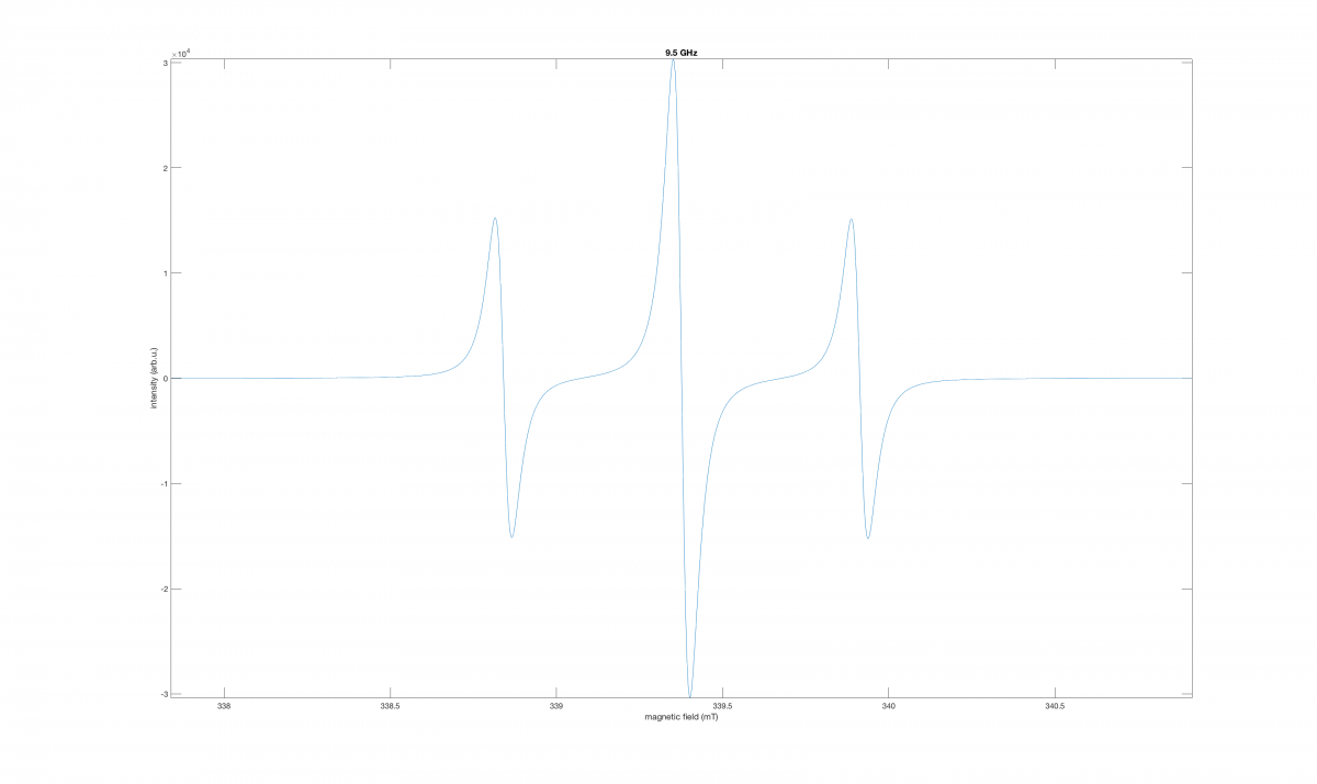
This should yield something that looks like:

Importing Data

EasySpin has a function for doing this, called eprload(). The method used to import your data depends on the format in which your experimental data is saved:

• For Modern Bruker Spectrometer Data:

    [B,spc] = eprload('mydata');

• For Older Bruker Spectrometer Data:

    [B,spc] = eprload('myolddata.spc');
    [B,spc] = eprload('myolddata.par');

The function changes when you are trying to load a text file of data:

• For Data Stored in Text Files:

    [B,spc] = textread('mydata.txt','%f %f');

• Text Files with Header Information:

    [B,spc] = textread('mydata.txt','%f %f','headerlines',17)

Creating a Simulation

The central concept to constructing a simulation with EasySpin is defining a Spin System (Sys) and Experimental Parameters (Exp).

Spin System

There are a variety of components that factor into a Spin System.

Electron and Nuclear Spins

The spins can be defined with Sys.S() according to the following:

    Sys.S = 1/2;            % one electron spin with S=1/2
    Sys.S = 5/2;            % an S=5/2 spin
    Sys.S = [1/2, 1/2];     % two S=1/2 spins
    Sys.S = [1, 1, 1/2];    % two S=1 spins and one S=1/2 spin

If this is not specified, the default value is S = 1/2.

The Nuclei can be specified using Sys.Nucs() according to the following:

    Sys.Nucs = '1H';              % one hydrogen
    Sys.Nucs = '63Cu';            % a 63Cu nucleus
    Sys.Nucs = '59Co,14N,14N';    % a 59Co and two 14N nuclei

You can specify an arbitrary number of nuclei for this system. In order to specify the number of each type of nucleus, you must use Sys.n() :

    Sys.Nucs = '1H,13C';  % one class of 1H and one class of 13C
    Sys.n = [2 3];        % 2 protons and 3 carbon-13 spins

G-value

As you're on this page, you are probably aware that there are some considerations to be made about the kind of system (isotropic vs. anisotropic) we are simulating when specifying the g-value. For all purposes here, we will assume that it will always be isotropic. To specify this you must use Sys.g():

    Sys.g = 2.0023;

This actually is not necessary, since the default is set to 2.0023... for all inputs. Still worth mentioning!

Hyperfine Coupling Constants and Number of Equivalent Nuclei

These are specified in MHz in EasySpin. No worries, though because EasySpin has a function that allows us to convert mT (or Gauss) into MHz:

    A_MHz = mt2mhz(A_mT);    % mT -> MHz conversion
    A_MHz = mt2mhz(A_G/10);  %  G -> MHz conversion (1 G = 0.1 mT)

Consider the following system, in which you have a hydrogen atom with a 10 MHz coupling to the unpaired electron and a 13C atom with a 12 MHz coupling:

    Sys.Nucs = '1H,13C'; % Defines the Hydrogen nucleus and the Carbon-13 nucleus
    Sys.A = [10 12]; % MHz... Defines the HFCC

To specify the number of equivalent nuclei, Sys.n() is used, as shown in the following examples:

For a single proton:

    Sys.Nucs = '1H';
    Sys.n = 1;
    Sys.A = 5.3;

For two equivalent protons (with identical hyperfine coupling constants):

    Sys.Nucs = '1H';
    Sys.n = 2;
    Sys.A = 5.3;

For something more complex (such as the naphthalene radical anion, which contains two sets of 4 equivalent nuclei):

    Sys.Nucs = '1H,1H';
    Sys.n = [4 4];
    Sys.A = [-14 -5];

Line Width

To specify the line width, EasySpin uses Sys.lwpp(). This gives the peak-to-peak line width. It should be noted here that the unit used for Line Widths is mT!!! For peak-to-peak line widths:

    Sys.lwpp = [0 0.03]; % Gaussian and Lorentzian peak-to-peak line width, mT

There is another option Sys.lw():

    Sys.lw = [0 0.05]; % Gaussian (1st input) and Lorentzian (2nd input) FWHM (full width at half height), mT

Experiment Parameters

There are a variety of fields that you can/must specify before you can get your simulated spectrum.

Microwave Frequency

The microwave frequency must be given in units of GHz. This can easily be defined with the following:

    Exp.mwFreq = 9.385;  % X-band

Field Range/Sweep Width

This is an optional step. If omitted, EasySpin will attempt to determine a Sweep Width large enough to accommodate the entire spectrum, but this can fail.

There are two ways to enter the magnetic field sweep width. Either give the center field and the sweep width (in mT) in Exp.CenterSweep():

    Exp.CenterSweep = [340 80]; % in mT

As an alternative, you can specify the lower and upper limit of the sweep range (again in mT) in Exp.Range():

    Exp.Range = [300 380];      % in mT

Number of Points

Again, an optional step. It is not required to be a power of 2 for EasySpin.

    Exp.nPoints = 5001;

Harmonic

You can set the harmonic that EasySpin will calculate, meaning either the Absorption or a derivative. This is specified with Exp.Harmonic():

    Exp.Harmonic = 0; % absorption spectrum, direct detection
    Exp.Harmonic = 1; % first harmonic (default)

Running the Simulation

Once you are ready to run the simulation, you simply have to call the garlic() function on your Spin System variable (Sys) and Experimental Set-up Variable (Exp):

    garlic(Sys,Exp);

Multiple Species in one Simulation

EasySpin can handle this fairly well, by simply defining a second Spin System:

   Sys1.g = 2;
   Sys1.lwpp = 1;     	
   Sys1.weight = 2;
   Sys2.g = 2.1;
   Sys2.lwpp = 0.8;
   Sys2.weight = 1;
   Exp.mwFreq = 9.5;
   Exp.Range = [300 360];
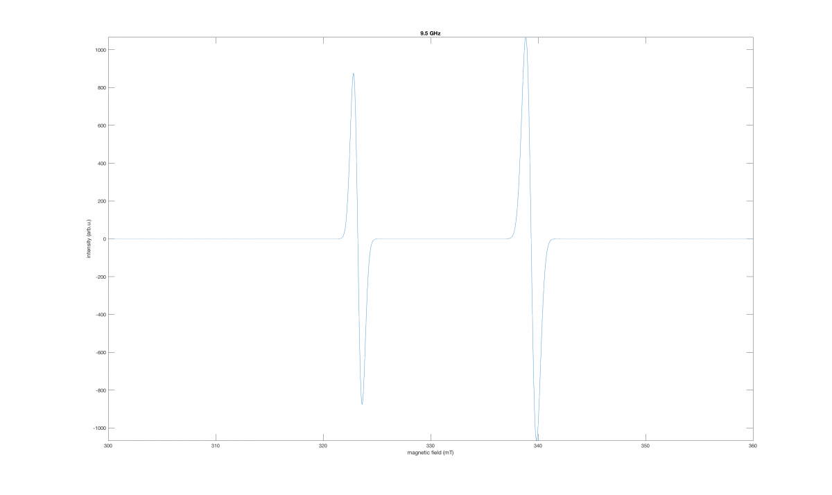
   garlic({Sys1,Sys2},Exp);