EPR Simulations with EasySpin

Installing Software

EasySpin is a MATLAB toolkit, so you must first install MATLAB. You can sign up for a trial version by entering your email here .

1) Create your MathWorks account and follow the prompts...

2) Once you're on the download page, choose the installer that meets your OS.

3) Once this is downloaded, click on it to run the installation software.

4) Once prompted, sign into your MathWorks account and select the license you would like to download and install for the trial.

5) Select the products you would like to download and install. (I left all of them selected.)

6) Let the installation complete... You now have MATLAB.

To get EasySpin, you must download it here (click on the "Get Latest Version" button).

7) Now, "Extract" or Unzip the files you have downloaded. (Location doesn't matter, entirely up to you.)

8) Now, launch MATLAB. You have to "connect" EasySpin to MATLAB...

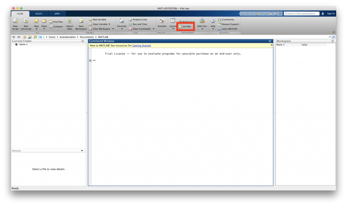
9) To do this, you must click on Home->Set Path (see picture below)

10) Click on "Add Folder" and select the EasySpin subfolder, called easyspin (easyspin-x.y.z/easyspin). Then click Save.

This should have made it possible for MATLAB to communicate with EasySpin. You can test this by typing easyspin into the MATLAB command prompt... Happy simulating!

Overview

This page serves as a resource to assist those trying to simulate EPR spectra with the EasySpin MATLAB package.

We should start out with a simple example, to see what kind of input EasySpin requires. Then, we will talk about the details regarding the parameters encountered in the example.

A simple example simulation:

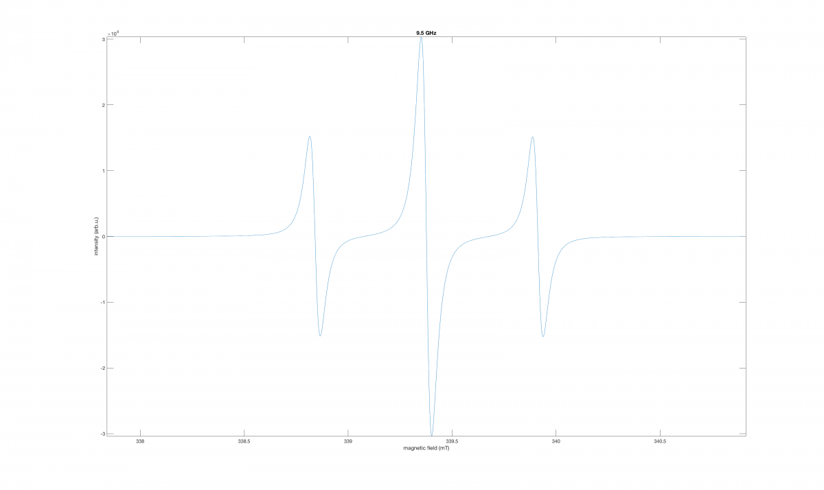
    Sys = struct('g',2,'Nucs','1H','n',2,'A',15,'lwpp',[0 0.05]);
    Exp = struct('mwFreq',9.5);
    garlic(Sys,Exp);

This should yield something that looks like:

Importing Data

EasySpin has a function for doing this, called eprload(). The method used to import your data depends on the format in which your experimental data is saved:

For Modern Bruker Spectrometer Data:

    [B,spc] = eprload('mydata');

For Older Bruker Spectrometer Data:

    [B,spc] = eprload('myolddata.spc');
    [B,spc] = eprload('myolddata.par');

The function changes when you are trying to load a text file of data:

For Data Stored in Text Files:

    [B,spc] = textread('mydata.txt','%f %f');

Text Files with Header Information:

    [B,spc] = textread('mydata.txt','%f %f','headerlines',17)

Creating a Simulation

The central concept to constructing a simulation with EasySpin is defining a Spin System (Sys) and Experimental Parameters (Exp).

Spin System

There are a variety of components that factor into a Spin System.

Electron and Nuclear Spins

The spins can be defined with Sys.S() according to the following:

    Sys.S = 1/2;            % one electron spin with S=1/2
    Sys.S = 5/2;            % an S=5/2 spin
    Sys.S = [1/2, 1/2];     % two S=1/2 spins
    Sys.S = [1, 1, 1/2];    % two S=1 spins and one S=1/2 spin

If this is not specified, the default value is S = 1/2.

The Nuclei can be specified using Sys.Nucs() according to the following:

    Sys.Nucs = '1H';              % one hydrogen
    Sys.Nucs = '63Cu';            % a 63Cu nucleus
    Sys.Nucs = '59Co,14N,14N';    % a 59Co and two 14N nuclei

You can specify an arbitrary number of nuclei for this system. In order to specify the number of each type of nucleus, you must use Sys.n() :

    Sys.Nucs = '1H,13C';  % one class of 1H and one class of 13C
    Sys.n = [2 3];        % 2 protons and 3 carbon-13 spins

G-value

As you're on this page, you are probably aware that there are some considerations to be made about the kind of system (isotropic vs. anisotropic) we are simulating when specifying the g-value. For all purposes here, we will assume that it will always be isotropic. To specify this you must use Sys.g():

    Sys.g = 2.0023;

This actually is not necessary, since the default is set to 2.0023... for all inputs. Still worth mentioning!

Hyperfine Coupling Constants and Number of Equivalent Nuclei

These are specified in MHz in EasySpin. No worries, though because EasySpin has a function that allows us to convert mT (or Gauss) into MHz:

    A_MHz = mt2mhz(A_mT);    % mT -> MHz conversion
    A_MHz = mt2mhz(A_G/10);  %  G -> MHz conversion (1 G = 0.1 mT)

Consider the following system, in which you have a hydrogen atom with a 10 MHz coupling to the unpaired electron and a 13C atom with a 12 MHz coupling:

    Sys.Nucs = '1H,13C'; % Defines the Hydrogen nucleus and the Carbon-13 nucleus
    Sys.A = [10 12]; % MHz... Defines the HFCC

To specify the number of equivalent nuclei, Sys.n() is used, as shown in the following examples:

For a single proton:

    Sys.Nucs = '1H';
    Sys.n = 1;
    Sys.A = 5.3;

For two equivalent protons (with identical hyperfine coupling constants):

    Sys.Nucs = '1H';
    Sys.n = 2;
    Sys.A = 5.3;

For something more complex (such as the naphthalene radical anion, which contains two sets of 4 equivalent nuclei):

    Sys.Nucs = '1H,1H';
    Sys.n = [4 4];
    Sys.A = [-14 -5];

Line Width

To specify the line width, EasySpin uses Sys.lwpp(). This gives the peak-to-peak line width. It should be noted here that the unit used for Line Widths is mT!!! For peak-to-peak line widths:

    Sys.lwpp = [0 0.03]; % Gaussian and Lorentzian peak-to-peak line width, mT

There is another option Sys.lw():

    Sys.lw = [0 0.05]; % Gaussian (1st input) and Lorentzian (2nd input) FWHM (full width at half height), mT

Experiment Parameters

There are a variety of fields that you can/must specify before you can get your simulated spectrum.

Microwave Frequency

The microwave frequency must be given in units of GHz. This can easily be defined with the following:

    Exp.mwFreq = 9.385;  % X-band

Field Range/Sweep Width

This is an optional step. If omitted, EasySpin will attempt to determine a Sweep Width large enough to accommodate the entire spectrum, but this can fail.

There are two ways to enter the magnetic field sweep width. Either give the center field and the sweep width (in mT) in Exp.CenterSweep():

    Exp.CenterSweep = [340 80]; % in mT

As an alternative, you can specify the lower and upper limit of the sweep range (again in mT) in Exp.Range():

    Exp.Range = [300 380];      % in mT

Number of Points

Again, an optional step. It is not required to be a power of 2 for EasySpin.

    Exp.nPoints = 5001;

Harmonic

You can set the harmonic that EasySpin will calculate, meaning either the Absorption or a derivative. This is specified with Exp.Harmonic():

    Exp.Harmonic = 0; % absorption spectrum, direct detection
    Exp.Harmonic = 1; % first harmonic (default)

Running the Simulation

Once you are ready to run the simulation, you simply have to call the garlic() function on your Spin System variable (Sys) and Experimental Set-up Variable (Exp):

    garlic(Sys,Exp);

Multiple Species in one Simulation

EasySpin can handle this fairly well, by simply defining a second Spin System:

   Sys1.g = 2;
   Sys1.lwpp = 1;     	
   Sys1.weight = 2;
   Sys2.g = 2.1;
   Sys2.lwpp = 0.8;
   Sys2.weight = 1;
   Exp.mwFreq = 9.5;
   Exp.Range = [300 360];
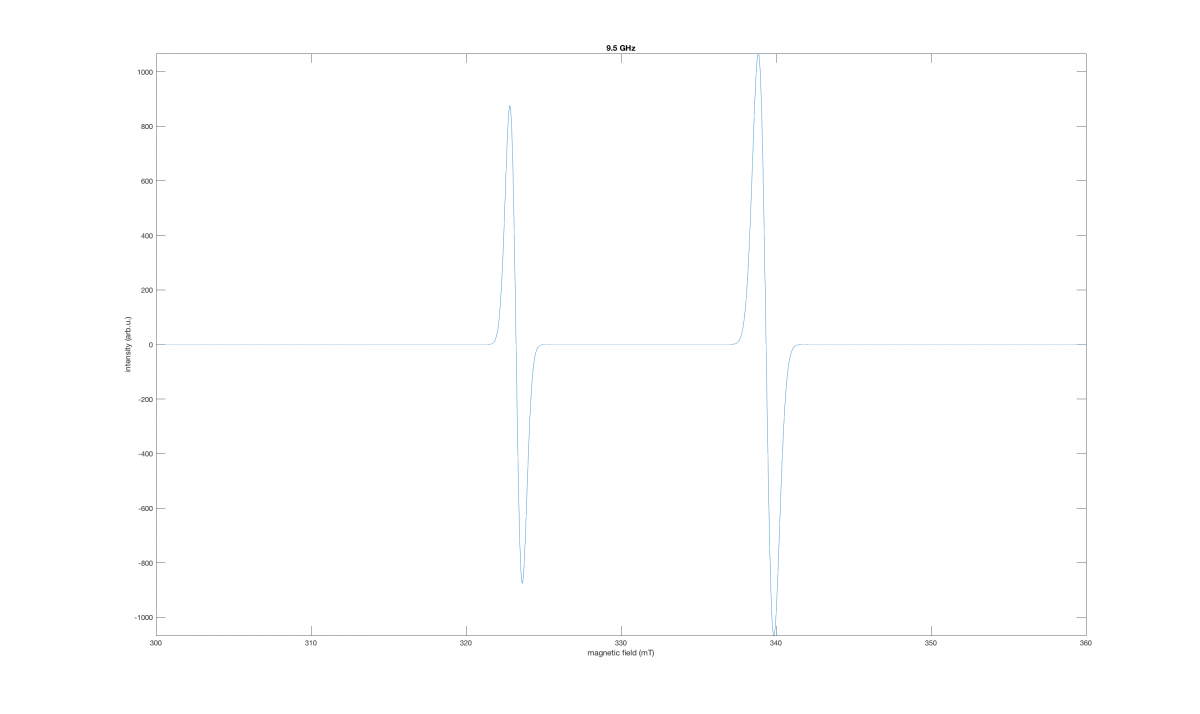
   garlic({Sys1,Sys2},Exp);

Fitting EPR Spectra with EasySpin

The Fitting Function

In order to fit an EPR Spectrum, EasySpin uses a function called esfit(). The general structure of this command is as follows:

   esfit('simulation function',spc,Sys0,Vary,Exp)

An explanation of the parameters of the esfit() function:

'simulation function' is the EasySpin simulation function that will be used for the fit. For fast-motion, isotropic EPR spectra the function will be garlic as discussed above.

spc is the array containing the experimental spectral data

Sys0 is a structure containing the magnetic parameters of the spin system. These parameters are used as first guesses in the fitting procedure. For multiple systems, this will be a list: {Sys1, Sys2}.

Vary is a structure similar to Sys0 containing the search ranges of the parameters that should be fitted. For a multicomponent fit, this is again a list of structures, one for each component: {Vary1, Vary2}. This should have the same defined parameters as Sys0.

Exp is a structure containing the experimental parameters for the simulation function, as discussed above.

Loading the Experimental Spectrum

The first step is to import the experimental data. This is done in the same fashion as we did earlier.

   [B, spc] = textread('filename.txt', '%f %f', 'header', number of header lines)

Initial Set of Parameters

   Sys0.g = 2.0;
   Sys0.lw = 1;

Parameter Search Range

This allows us to tell esfit what to change in Sys0 by utilizing the Vary class.

   Vary.lw = 0.3

These variations are the original value defined in Sys0 +/- the value defined in Vary.

You should vary no more than 4 parameters at once. As the number of degrees of freedom increases, the difficulty of the fit dramatically increases.

Launching the Fitting Graphical User Interface (GUI)

Now that you have defined all of the parameters needed to run the fit of your experimental spectrum, you simply need to call the esfit() function:

   esfit('simulation function',spc,Sys0,Vary,Exp)

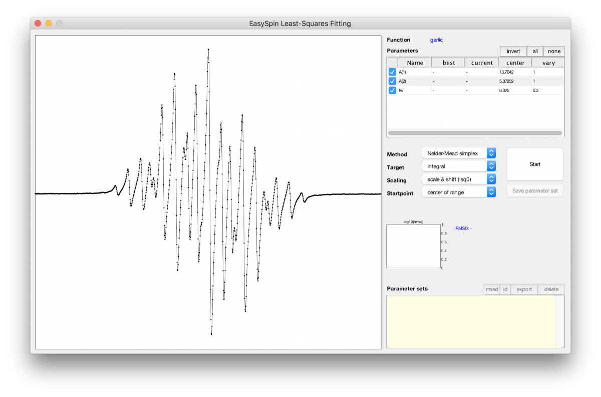
This will launch the GUI, pictured below. This can be very daunting at first, but we will take a look at what all of these parameters mean.

Fitting Methods

Here, we will take a look at what the various optimization algorithms and target functions do.

Optimization Algorithms

There are five optimization algorithms in EasySpin:

Neider/Mead Downhill Simplex
Levenberg/Marquardt Algorithm
Monte Carlo Random Search
Genetic Algorithm
Particle Swarm/Systematic Grid Search

Neider/Mead Downhill Simplex and Levenberg/Marquart Algorithm are both local search algorithms, which begin with the given starting parameters and then work their way down a nearby valley of the parameter space to find a minimum. Both are relatively fast methods, but there are some general differences. The downhill simplex is slower than the Levenberg/Marquardt, but it is less likely to get stuck in a local minimum.

The remaining three algorithms are global search methods: they do not have a starting set of parameters, but use a variety of sets distributed over the entire parameter search space.

The Monte Carlo method simply performs a series of random trial simulations and then picks the best one. It is very inefficient. The systematic grid searches better because it covers the parameter space with a grid and then does simulations for each knot of the grid in random order. No point is simulated twice and this is a more efficient method than the Monte Carlo search. But, if the minimum is between two grid points, it will never be found.

The genetic algorithm makes simulations for several (N) parameter sets (called a population), computes the fitting error (called the fitness) for all of them, and then proceeds to generate N new parameter sets from the old ones using mechanisms like mutation, cross-over, and reproduction. This way, a new generation of parameter sets is procreated, as in biological evolution. The benefit of this algorithm is that if a good parameter is encountered, then it is likely to propagate down the generations and across the population.

Target Function

The second important setting is the target function. 'esfit' computes the error of the simulated spectrum using the root-mean-square-deviation (rmsd, which is the square root of the mean of the squared standard deviations), where the deviation is the difference between the simulated and experimental spectra.

Fitting speed can often be increased if the spectra are not directly used, that is, if their integrals or similar transforms are used instead. The options in EasySpin are as follows

Data As Is
Integral
Double Integral
First Derivative
Fast Fourier Transform

A Guided Tutorial

In order to see how all of the previous topics are involved in the EPR Simulation Process, we will walk through a guided tutorial where we will simulate real experimental data.

This tutorial requires the following input files:

General Structure of the Template File

    close all;  This line closes any pre-existing MATLAB Figures. 
    clear all;  This line clears all pre-existing variable definitions.

    [B,spec1] = textread('filename.txt', '%f %f');

This line defines the magnetic field (B) in units of the experimental spectrum (spec1). Recall that EasySpin uses units of mT, so you will have to convert your experimental spectrum if it was saved in units of Gauss. Here %f is referred to as a string formatter, allowing the textread() function to know that the experimental data is in "floating point decimal" format - indicating that the data is numerical with a variable position of the decimal point.

The next lines define our simulation system - here identified as M :

    M.S = System Spin; Define the spin of our system.
    M.Nucs = 'nuclei'; Define any nuclei present/coupled to the spin.
    M.g=[g-value(s)]; Define the principle g value or values for the system. (It's not always 2.0023.....)
    M.A =[Hyperfine Coupling Constant (in mHz)]; Define any hyperfine couplings present in the system (should have the same shape as M.Nucs)
    M.lwpp=[0.1 0.1]; % Defaults to units of what we are sweeping (mT/MHz field/frequency) Define our line width broadening - 
                                   % Note that this is in the format of a Voigt curve with [Gaussian_Component Lorentzian_Component].

Next we have to set-up the Experimental Parameters for the simulation:

    Exp=struct('mwFreq',x.xx,'nPoints',xxxx,'Range',[xx.xx xx.xx]);  Define our magnetic field window for the simulation - which can be easily obtained from the experimental set-up. 
    Note: nPoints should match the number of points in the experimental data file.
    Exp.Temperature = x; Define the temperature at which the experimental spectrum was collected.

We then run the simulation using a specific regime function (garlic, pepper, etc.):

    [B,simul1]=regimefunction(M,Exp);

Finally, we can apply a baseline correction to our experimental spectrum or an intensity correction to our simulated spectrum:

    y=spec1+b % Baseline Correction/y-shift
    y2=simul1*k % Intensity correction for simulated data.

Important Note: the template MATLAB file provided above is currently saved as a '.txt' file (so I could upload it to the Wiki server) - you will need to change this extension to '.m' in order to run in MATLAB.

Simple Example: DPPH

DPPH is a common standard used in EPR. This has a well-characterized spectrum, which makes identification of the principle g-value and hyperfine coupling constant very easy.

We will now walk through the steps of simulating this spectrum.

Create a folder named "DPPH". Add to this folder both the experimental data file (DPPH.txt) and a copy of the MATLAB template file.
Open your template file and save it as something like DPPH_simulation.m
We will now adjust some lines of the original template to begin our simulation.
- Change filename.txt to DPPH.txt

    [B,spec1] = textread('DPPH.txt', '%f %f');

We are dealing with a lone free radical in DPPH without hyperfine coupling, so we must change System Spin to 1/2 and comment out M.Nucs and M.A

    M.S = 1/2;
    %M.Nucs = 'nuclei'; 
    %M.A =[Hyperfine Coupling Constant (in mHz)];

DPPH has a well-characterized principle g-value of 2.0036, so insert this value

    M.g=[2.0036];

Play with the peak-peak line broadening.

    M.lwpp=[0.1 0.1];

Set the experimental parameters to:

     Exp=struct('mw Freq',x.xx,'nPoints',xxxx,'Range',[xx.xx xx.xx]);

Set the experimental temperature to 298 K:

    Exp.Temperature = 298;

We are in the fast-motion, liquid regime, so we will use garlic

    [B,simul1]=garlic(M,Exp);

Play with the baseline and intensity corrections. (Hint: This spectrum requires no baseline and has an intensity correction of 0.05.)

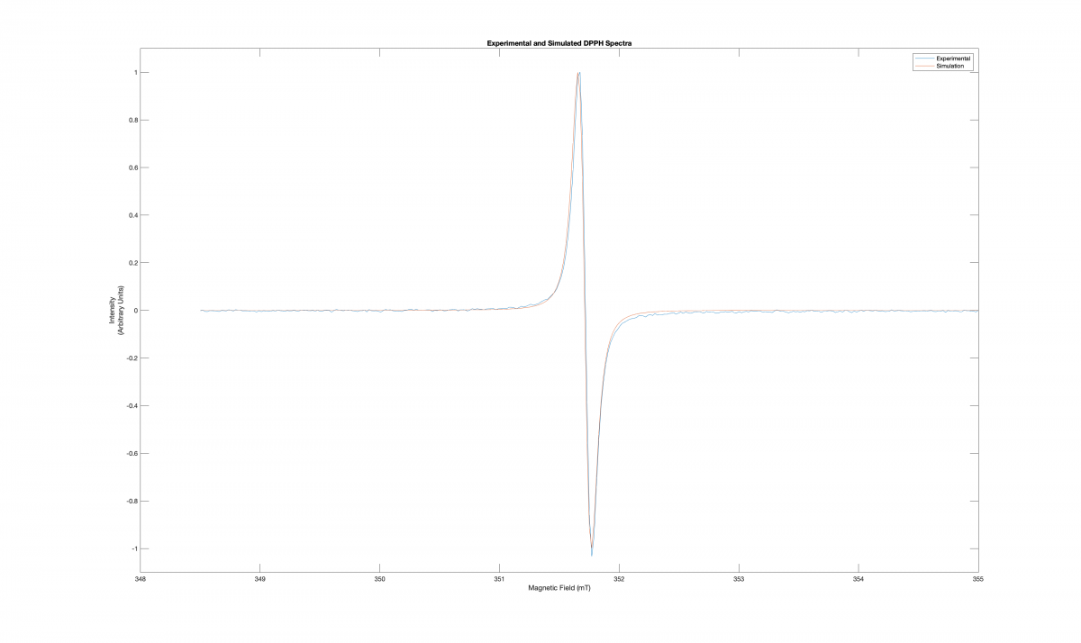
Your final output should look like the following figure:

Example 2: TEMPO

Simulating the Spectrum

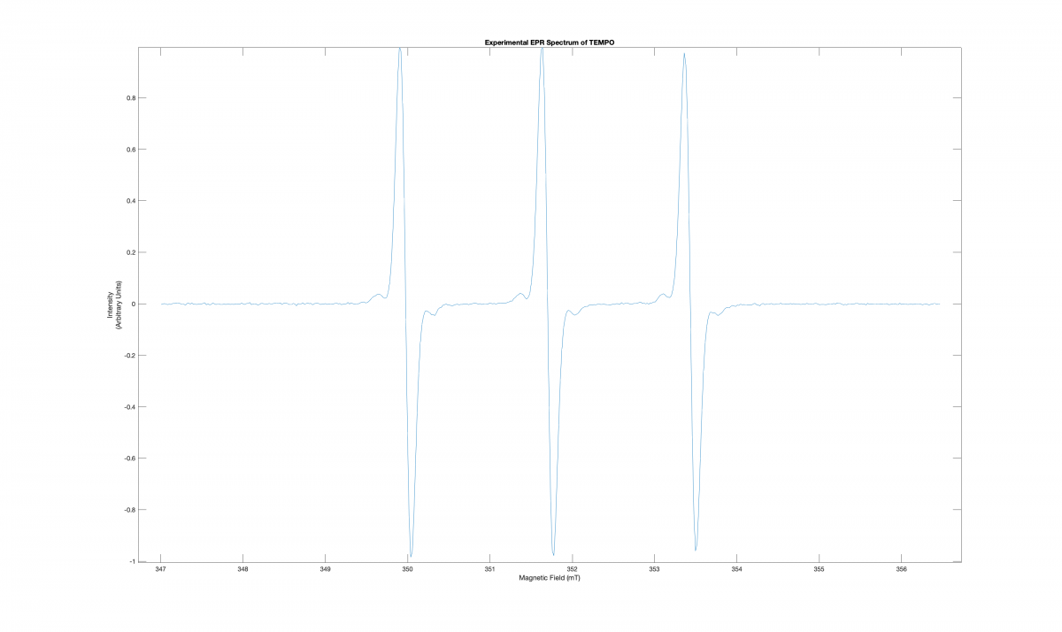
Structure of 2,2,6,6-Tetramethylpiperidinyloxyl (TEMPO)

TEMPO is a nitroxide that is commonly encountered in the field of EPR. Its spectrum serves as an excellent example of an isotropic signal displaying hyperfine coupling. This adds another layer of difficulty to the procedure used in the DPPH spectrum above. The hyperfine coupling arises from delocalization of the radical across both the oxygen and nitrogen atoms. The experimental spectrum is displayed below. Nitrogen-14 has nuclear spin of I = 1, which accounts for the three lines in the spectrum. Note that there are also some satellite peaks located on each side of each of the three peaks.

Now, let's get started with the simulation:

Create a folder named "TEMPO". Add to this folder both the experimental data file (TEMPO.txt) and a copy of the MATLAB template file.
Open your template file and save it as something like DPPH_simulation.m
Modify the code and see how well you can simulate the experimental spectrum, taking note of the following experimental parameters:
- Microwave Frequency: 9.869 GHz
- Number of Points: 485
- Field Range: 347 - 356.5 mT
- Temperature: 298 K

TEMPO is an organic radical, so you can safely guess that the principle g-value will be around 2.0. If you'd rather handle this directly, you can utilize the following relationship between the magnetic field, microwave radiation, and g-value to calculate a g-value to use for your guess:

As previously mentioned, TEMPO exhibits hyperfine coupling. This means that you will have to define a nucleus in the M.A line. Recall from above that EasySpin thinks about Hyperfine Couplings in units of MHz. If you prefer to think about these values in terms of Magnetic Field units (Gauss or milliTesla), you can use the mt2mhz() to wrap your input as follows:

    M.A = [mt2mhz(A in mT)];

Note that you can estimate the hyperfine splitting directly from the spectrum and then convert to MHz with the following equation:

Play with the Hyperfine Coupling Constant (A), line width (lwpp), g, and the scaling factor until you have a sufficient fit of the main triplet signal. Once you've successfully simulate the triplet, you may move onto the satellite peaks. (Hint: what splits a single signal into two signals?)

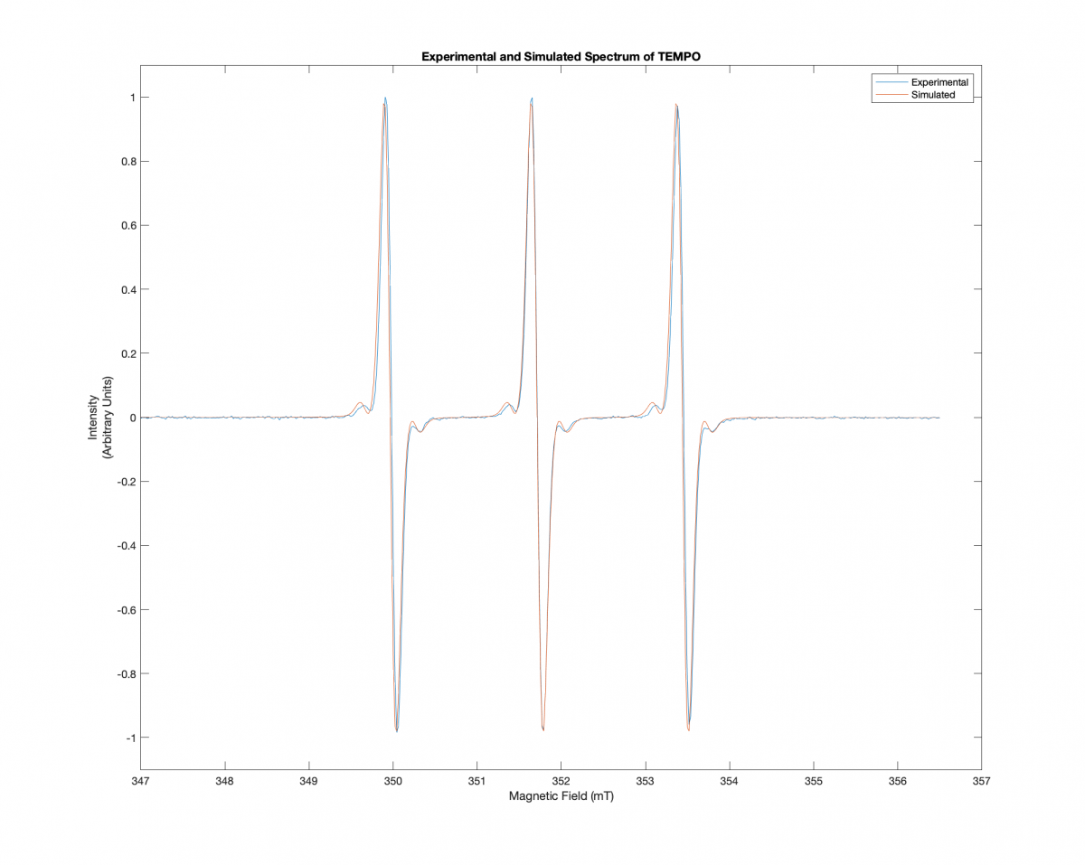
Once you've got a decent simulation, you should see something like this:

Fitting the Spectrum with EasySpin's esfit Function

Now that you've obtained an approximate simulation in EasySpin, we can exploit its robust fitting functionality. At the bottom of the template file, you should see the following lines:

     Vary.parameter = [Variation Range]; 
     esfit('regime function', spec1, M, Vary, Exp);

The first line allows us to specify a certain parameter that we are interested in varying (such as the Hyperfine Coupling A), as well as the range we would like to restrict the variation algorithm to. The second line calls the fitting function esfit. This function takes the parameters of the regime function (in this case we will use garlic()), our experimental spectrum (spec1), the simulation system (M), our varied parameters (Vary), and our Experimental Parameters (Exp). (More on esfit above...)

Replace these lines with the following lines:

Vary.A = [5, 5]; Vary.lwpp = [0.01 0.01]; esfit('garlic', spec1, M, Vary, Exp);

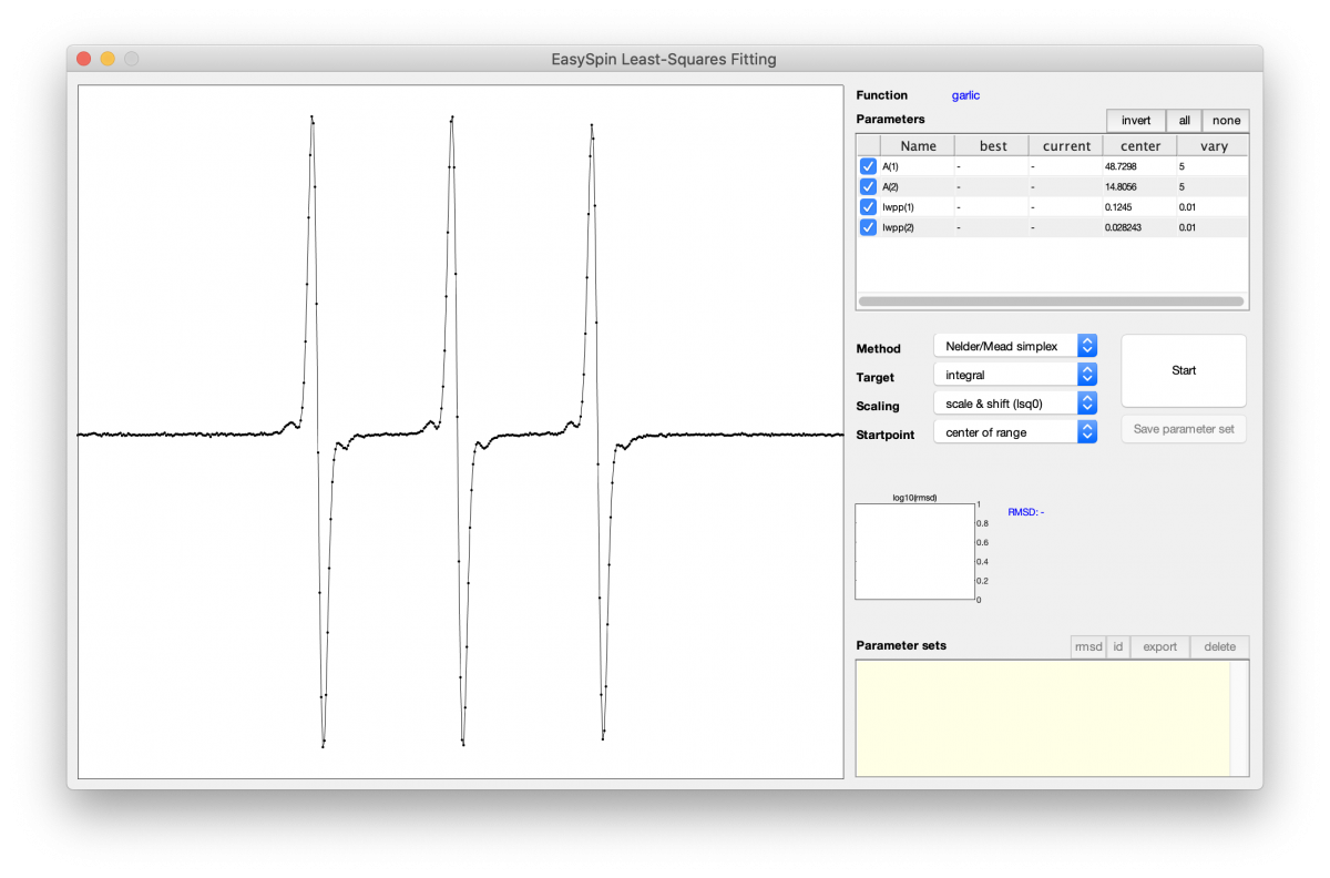
Now execute the code and you should see the following window:

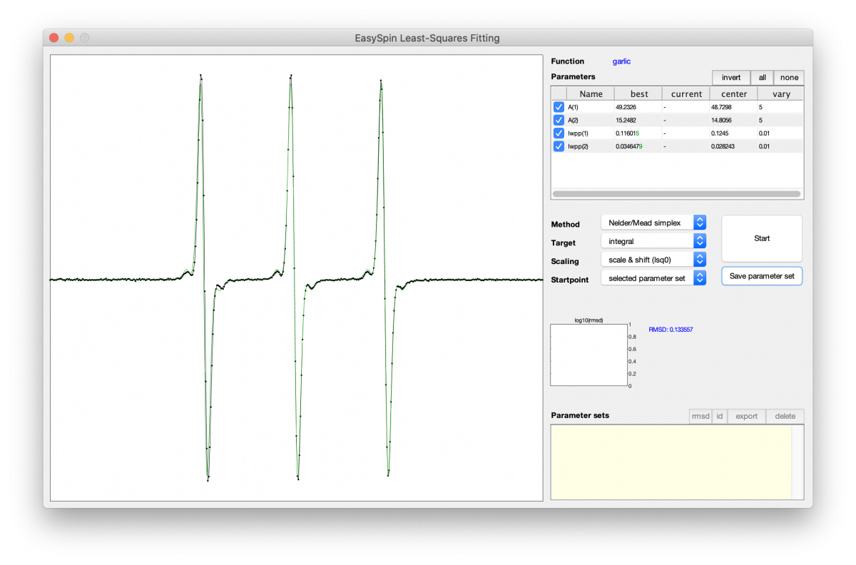
Feel free to play around with these different parameters. They are explained in detail above. When you're ready to run the fitting procedure, select the "Start" button and watch the fitting algorithm work its magic! If you obtained a successful fit, you will see a green spectrum like this:

If you'd like to save your parameters, you can do so selecting "Save Parameter Set", allowing you to set these parameters as the starting point for additional fittings as necessary. You can also export these parameters to your workspace, allowing you to update your original simulation code.

Congratulations on completing the EPR Tutorial! By no means is this tutorial exhaustive, it intends to serve as an introduction to the world of EPR simulation. You're now prepared to go into the lab, collect a spectrum, and simulate some data!