Difference between revisions of "HCl Vibrational-Rotational Spectroscopy"
Jump to navigation
Jump to search
| Line 41: | Line 41: | ||
|} | |} | ||
| − | : | + | :a) Make a plot, m-value verses freq (in 1/cm) for H<sup>35</sup>Cl data; this will NOT be a straight line but a polynomial curve. |
| + | :b) fit a second order polynomial to this data... ie y= ax<sup>2</sup> + bx +c, and note the values for a, b, and c in your notes (lab notebook preferred). | ||
| + | :c) During our last lab period you were given a Shoemaker, etc. handout (???) that discussed this lab activity. Eq. 9 was: | ||
| + | |||
| + | <div> align="center"'' ṽ = ṽ<sub>o</sub> + (2B<sub>e</sub> - 2 α<sub>e</sub>) m - α<sub>e</sub> m<sup>2</sup> ''</div> | ||
::https://en.wikipedia.org/wiki/Isotopes_of_chlorine | ::https://en.wikipedia.org/wiki/Isotopes_of_chlorine | ||
Revision as of 14:24, 26 March 2020
Adapted from Experiment #38 (Shoemaker, Garland, Nibler, 1989)
See Chapter 8 (Engel), more will be presented in lecture...
Sample Preparation
- a) Pull the HCl (g) off the headspace of a bottle of concentrated HCl using a 60 mL syringe.
- b) deliver the HCl (g) to the gas-sampling IR cell.
IR Gas-Phase Data Collection
- a) Collect data using the highest resolution.
- b) average 32 scans (both background and sample)
- c) Save-As...
- (A complete set of data can be found here.)
Spectral Analysis
- a) load IR data into Igor or Excel.
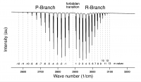
- b) Use the cursor tool to tabulate the H35Cl and H37Cl data into separate columns,
- c) Assign an "m-value" to each transition (note the 'm=0' forbidden transition) with the help of the following graphic (click to make bigger).

Data Analysis
Okay, so you should now have a table, probably in Excel but if you know how to do it in Igor then great (Igor does not offer any advantages here) with heading like this:
| m-value | H35Cl | H37Cl |
| -12 | XXXX | YYYY |
| -11 | XXXX | YYYY |
| -10 | XXXX | YYYY |
| -9 | XXXX | YYYY |
| ... | ... | ... |
| +1 | XXXX | YYYY |
| +12 | XXXX | YYYY |
| +13 | XXXX | YYYY |
- a) Make a plot, m-value verses freq (in 1/cm) for H35Cl data; this will NOT be a straight line but a polynomial curve.
- b) fit a second order polynomial to this data... ie y= ax2 + bx +c, and note the values for a, b, and c in your notes (lab notebook preferred).
- c) During our last lab period you were given a Shoemaker, etc. handout (???) that discussed this lab activity. Eq. 9 was:
align="center" ṽ = ṽo + (2Be - 2 αe) m - αe m2
- Reduced mass, "mu" = (m1*m2)/(m1+m2)
- 1H 1.007825 amu (99.9885%)
- 35Cl 34.968853 amu (75.78%)
- 37Cl 36.965903 amu (24.22%)
- conversion factor: 1.66054e-27 kg/amu
4) Plot "m" (x) vs the frequency (y) and fit to a second order polynomial.
5) The second order polynomial will take the form of equation 9 from (Exp 38, Shoemaker), hence you can determine alphae, and then of Be.
6) Using equation 5 and 3, then solve for "r" the average internuclear separation.